This is the second post in of this series about feature engineering for recommendation systems. In the first part, we looked at counter and rate-based features and a few best practices related to writing them. In the second part (i.e., this post), we will look at a few more techniques and best practices for writing good counter/rate based features. And in the third and final part, we will look at more advanced kinds of features that work well for large neural networks.
As a reminder, the following four ideas were introduced in part 1:
- Choose the appropriate splits (for counter/rate features)…
- …but don’t make them too sparse
- Don’t forget to add context
- Dynamically match users and candidates
Let’s now look at a few more best practices and techniques for working counter features.
5. Max/min pool related “options”
Imagine you are building a dating product as part of which you need to recommend potential other users to viewer. You have an insight that people prefer to date people with similar hobbies/interests. So you build a rating feature to capture people’s preference towards certain hobbies — the feature will measure “the acceptance rate of the viewer on people who have a hobby H” to capture users’ affinity towards a particular hobby. All good.
But most users have multiple hobbies. When evaluating a candidate user for the viewer, which of their many hobbies should be used to compute the viewer’s affinity?
A very simple and successful approach is to compute it for all their hobbies and take a max over those. In other words, the feature’s definition becomes:
feature(viewer, candidate) = max over all hobbies H of candidate (accept rate of viewer on people with hobby H)
This is a very common pattern, especially while writing features to capture the affinity of people towards specific topics / categories / hobbies / tags or other similar concepts involving a fan out. Further, max is just one way of combining these many affinities. In empirical experience, min and mean also work very well. In fact, they all capture different kinds of information, so it’s common to have all three of these present. In the above example of dating recommendation, we will throw in three versions of this feature - one with max pooling, one with min pooling, and one with mean pooling.
6. Use Wilson intervals to normalize rate features
Rate features are smarter than simple counter features because they capture not only raw volume but relative preference. For instance, if a particular old product has been around longer, it would have been shown to more people => a counter feature like “number of times it has been bought” will be high. But that feature isn’t well-behaved because it is biased towards older content. In comparison, if there was a new product that has been shown to a few hundred people only but has a much higher purchase rate, it might very well be a better candidate to show.
However, this same logic can also backfire if the denominators are very small. Let’s imagine this scenario - in an EdTech product, a new video was just uploaded, and it was recommended to three people. But by sheer chance/variance, none of those three people liked it. The value of the rate feature will be 0/3, which is equal to zero. So this zero value of the feature may convince the whole model to believe that this video isn’t relevant. However, this is a mistake because our estimate of zero is very noisy — had it been shown to some other three users, its value very well might have been 3/3. Obviously, the features stabilize as they get shown to more users, but when the denominators are too small, they are not yet very stable.
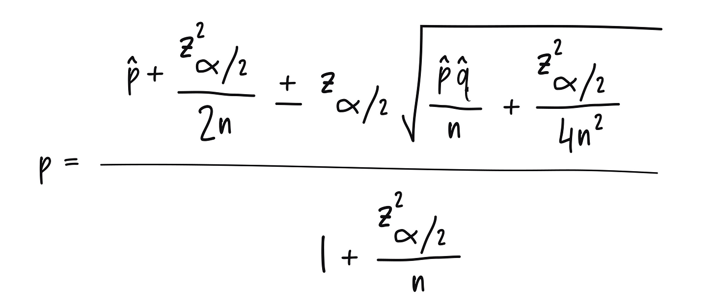
The best way to handle this is to normalize the rate feature somehow. There are many ways of doing that — the most common being additive normalization. However, I prefer Wilson confidence based normalization the most.

Don’t worry if the formula looks scary — it’s a relatively simple and fast calculation. More importantly, it is grounded in actual statistics — given n samples so far and an observed rate of p, it tells us the exact confidence interval bounds on the true rate. There is some value in throwing both the upper bound and the lower bound as a feature (i.e., two features per rate variable). Either way, whatever technique you choose, please normalize your rate features for the best results.
7. Use multiple rolling time windows
People’s preferences evolve over time — for instance, I was into reading health books a few months earlier but now have shifted to entrepreneurship books. And so, the ideal book recommendations for me have also changed over time. Similar changes also happen at macro level — the demand for ACs shoots up in the hot summer months. Similarly, the inventory of things to be recommended also evolves over time — new products come in, and older products get discontinued. And these time relationships get even more complex — e.g., if a user bought a TV last week, it’s unlikely that they will be looking to buy another TV today. But if the same user purchased a bag of diapers, they may be looking to buy another bag of diapers today.
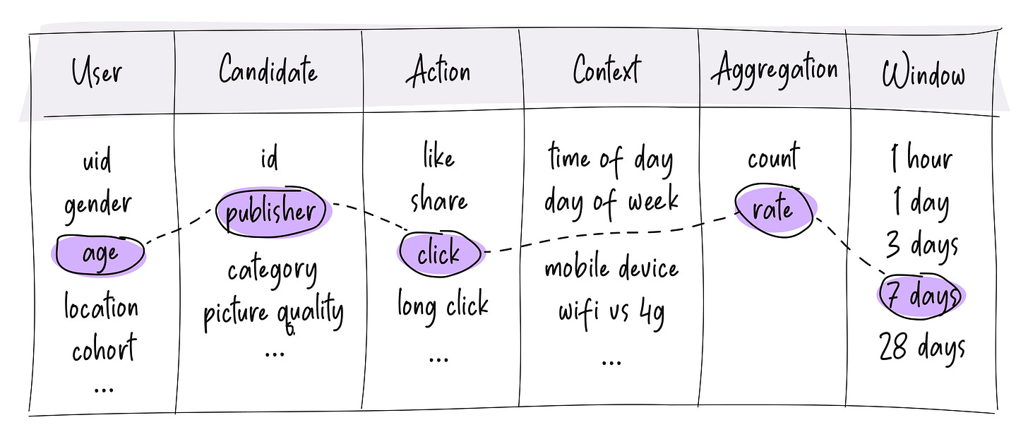
The technique to capture information from these complex time relationships turns out to be very simple - simply using multiple rolling time windows for any given counter/rate feature. For instance, say in an e-commerce product, we want to capture the user’s affinity towards the price of the products. So we build a feature to calculate their click rate on products of various prices. To capture time relationship information, all we will do is run this in multiple rolling windows like:
- User’s click rate on products of various prices in the last 1 days
- User’s click rate on products of various prices in the last 7 days
- User’s click rate on products of various prices in the last 28 days
While there is value in having multiple windows, there is also little point in having too many windows. Typically, a few windows are sufficient — say one or more for capturing changes at an hourly scale, another 1-2 splits for capturing changes at the daily level, another 1-2 windows for capturing changes at a weekly level, etc. With this, the table of counter features introduced in part 1 gets another column of time windows:

One crucial knob to tune is the duration of the longest time window — making it longer results in the feature capturing super long-term trends. But it also makes it a lot harder to compute/maintain/backfill. My recommendation is to stick with a 28-day window as the longest by default and go longer only if your specific product needs it. And even then, never go above 90 days or so. There are also privacy and data retention factors to be considered here. Either way, the highest order bit is just to have a few different rolling time windows.
8. Make your counter/rate features realtime
Finally, one of the greatest properties of counter features is how easily they can inject some realtime dynamism into model predictions. All you have to do is make your counter/rate features realtime. That way, even if the models themselves aren’t updating, shifts in counter feature distributions mirror evolving conditions and are able to make the final model predictions not drift as much (especially if you use somewhat robust models like GBDTs).
Now only this technique works in preventing serious model drift; it is in many ways superior to continuously re-training models in near-realtime:
- Counting things in a near-realtime manner is a much easier problem than continuously re-training your model in near-realtime. It’s much easier to scale even to very high write throughputs.
- It’s much cheaper from a computational cost point of view — updating models often requires calculating / propagating gradients, which in turn needs multiple floating point operations. Keeping counters up to date is often a single integer update.
- Much lower memory footprint — continuously re-training models require a lot of state to be kept in RAM. But counters can be maintained primarily on disk and still updated in near realtime at high write throughputs.
- If features are shared across multiple models (which often is the case), the cost of maintaining realtime counters gets amortized over multiple models which is not possible when models themselves are updating all the time.
Beyond a reasonable v1 model, bigger wins come from making the system more realtime instead of throwing in many more powerful features. A large edtech company that I spoke with earlier told us a similar story — they tried making some of their features realtime, and to simplify the “migration”, they threw away some of their most powerful/complex features. And they still saw huge metric wins. And this is not a one-off story — all production systems at top tech companies are built on top of realtime features today.
If you can take one thing away from this whole post it’s this — the new baseline for recommendation systems is not collaborative filtering but realtime counter/rate features with GBDT based models.
Conclusion
Unlike many other kinds of ML, most of the feature engineering for any recommendation or personalization system is based on counter or rate features. In this post, we reviewed some more techniques and best practices for encoding useful signals as counter and rate features. In the third and final part of this series, we will discuss how feature engineering is done for more advanced neural network-based recommendation systems — stay tuned!

