FANN: Vector Search in 200 Lines of Rust

Thanks to the rapid progress in AI/ML adoption, Vector databases are everywhere. And while they enable complex AI/ML applications, vector search itself is conceptually not that hard. In this post, we will describe how Vector databases work and also build a simple Vector Search library in under 200 lines of Rust code. All code can be found in this Github repo. The approach we use here is  based on a family of algorithms called "Locality Sensitive Hashing" used in the popular library annoy. This article's goal isn't to introduce a new fancy algorithm/library but to describe how vector search works using real code snippets.

But first, let's establish what vector search is.

Introduction to Vectors (aka Embeddings)

Complex unstructured data like docs, images, videos, are difficult to represent and query in traditional databases – especially if the query intent is to find "similar" items. So how can Youtube choose the best video to play next? Or Spotify customize the music queue according to your current song?

Advances in AI in early 2010s (starting with Word2Vec and GloVe) enabled us to build semantic representation of these objects in which they are represented as points in cartesian space. Say one video gets mapped to the point [0.1, -5.1, 7.55] and another gets mapped to the point [5.3, -0.1, 2.7]. The magic of these ML algorithms is that these representations are chosen such that they maintain semantic information –  more similar two videos, smaller the distance is between their vectors.

Note that these vectors (or more technically called as embeddings) don't have to be 3 dimensional - they could be and often are in higher dimensional spaces (say 128 dimensions or 750 dimensions). And the distance doesn't need to be euclidean distance either - other forms of distances, like dot products, also work. Either way, all that matters is the distances between them correspond to their similarities.

Now imagine that we have access to such vectors for all Youtube videos. How do we find the most similar video to a given starting video? Simple. Loop through all the videos, compute the distance between them and choose the video with the smallest distance - also known as finding the "nearest neighbours" of the query video. This will actually work. Except, as you can guess, a linear O(N) scan can be too costly. So we need a faster sub-linear way to find the nearest neighbours of any a query video. This is in general impossible - something has to give.

As it turns out, in practical situations, we don't need to find the nearest video - it'd also be okay to find near-enough videos. And this is where approximate nearest neighbor search algorithms, also known as vector search come in. The goal is to sub-linearly (ideally in logarithmic time) find close enough nearest neighbours of any point in a space. So how to solve that?

How to Find Approximate Nearest Neighbours?

The basic idea behind all vector search algorithms is the same – do some pre-processing to identify  points that are close enough to each other (somewhat akin to building an index). At the query time, use this "index" to rule out large swath of points. And do a linear scan within the small number of points that don't get ruled out.

However, there are lots of ways of approaching this simple idea. Several state-of-the-art vector search algorithms exist like HNSW (a graph that connects close-proximity vertices and also maintains long-distance edges with a fixed entry point). There exist open-source efforts like Facebook’s FAISS and several PaaS offerings for high-availability vector databases like Pinecone and Weaviate.

In this post, we will build a simplified vector search index over the given "N" points as follows:

1. Randomly take 2 arbitrary available vectors A and B.
2. Calculate the midpoint between these 2 vectors, called C.
3. Build a hyperplane (analog of a "line" in higher dimensions) that passes through C and is perpendicular to the line segment connecting A and B.
4. Classify all the vectors as being either “above” or “below” the hyperplane, splitting the available vectors into 2 groups.
5. For each of the two groups: if the size of the group is higher than a configurable parameter “maximum node size”, recursively call this process on that group to build a subtree. Else, build a single leaf node with all the vector (or their unique ids)

We thus use this randomized process to build a tree where every internal node is a hyperplane definition with the left subtree being all the vectors “below” the hyperplane and the right subtree being all the vectors “above”. The set of vectors are continuously recursively split until leaf nodes contain no more than “maximum node size” vectors. Consider the example in the following figure with five points:

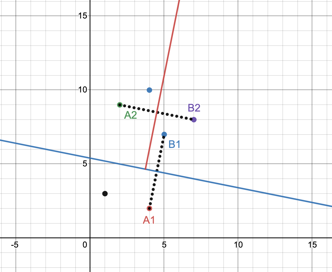
We randomly choose vectors A1=(4,2), B1=(5,7). Their midpoint is (4.5,4.5) and we build a line through the midpoint perpendicular to the line (A1, B1). That line is x + 5y=27 (drawn in blue) which gives us one group of 2 vectors, and one group of 4. Assume the “maximum node size” is configured to 2. We do not further split the first group but choose a new (A2, B2) from the latter to build the red hyperplane and so on. Repeated splits on a large dataset split up the hyperspace into several distinct regions as shown below.

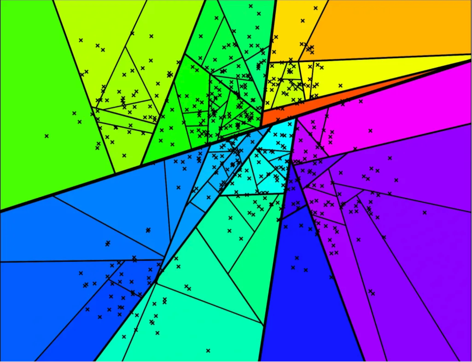
Each region here represents a leaf node and the intuition here is that points that are close enough are likely to end up in the same leaf node. So given a query point, we can traverse down the tree in logarithmic time to locate the leaf it belongs to and run a linear scan against all the (small number of) points in that leaf. This is obviously not foolproof - it's totally possible that points that are actually close enough get separated by a hyperplane and end up very far off from each other. But this problem can be tackled by building not one but many independent trees - that way if two points are close enough, they are far more likely to be in the same leaf node in at least some trees. At the query time, we traverse down all the trees to locate the relevant leaf nodes, take a union of all the candidates across all leaves, and do a linear scan on all of them.

Okay enough of theory. Let's start writing some code and first define some utilities for a Vector type in Rust below, for dot product, averaging, hashing, and squared L2 distance. Thanks to Rust's nice type system, we propagate the generic type parameter N to force all vectors in an index to be the same dimensionality at compile time.

#[derive(Eq, PartialEq, Hash)]
pub struct HashKey<const N: usize>([u32; N]);

#[derive(Copy, Clone)]
pub struct Vector<const N: usize>(pub [f32; N]);
impl<const N: usize> Vector<N> {
    pub fn subtract_from(&self, vector: &Vector<N>) -> Vector<N> {
        let mapped = self.0.iter().zip(vector.0).map(|(a, b)| b - a);
        let coords: [f32; N] = mapped.collect::<Vec<_>>().try_into().unwrap();
        return Vector(coords);
    }
    pub fn avg(&self, vector: &Vector<N>) -> Vector<N> {
        let mapped = self.0.iter().zip(vector.0).map(|(a, b)| (a + b) / 2.0);
        let coords: [f32; N] = mapped.collect::<Vec<_>>().try_into().unwrap();
        return Vector(coords);
    }
    pub fn dot_product(&self, vector: &Vector<N>) -> f32 {
        let zipped_iter = self.0.iter().zip(vector.0);
        return zipped_iter.map(|(a, b)| a * b).sum::<f32>();
    }
    pub fn to_hashkey(&self) -> HashKey<N> {
        // f32 in Rust doesn't implement hash. We use bytes to dedup. While it
        // can't differentiate ~16M ways NaN is written, it's safe for us
        let bit_iter = self.0.iter().map(|a| a.to_bits());
        let data: [u32; N] = bit_iter.collect::<Vec<_>>().try_into().unwrap();
        return HashKey::<N>(data);
    }
    pub fn sq_euc_dis(&self, vector: &Vector<N>) -> f32 {
        let zipped_iter = self.0.iter().zip(vector.0);
        return zipped_iter.map(|(a, b)| (a - b).powi(2)).sum();
    }
}

With these core utilities built out, let's also define how our Hyperplane will look:

struct HyperPlane<const N: usize> {
    coefficients: Vector<N>,
    constant: f32,
}

impl<const N: usize> HyperPlane<N> {
    pub fn point_is_above(&self, point: &Vector<N>) -> bool {
        self.coefficients.dot_product(point) + self.constant >= 0.0
    }
}

Next, let's focus on generating random hyper planes and building forest of nearest neighbor trees. How should we represent points within a tree?

We could directly store D-dimensional vectors inside leaf nodes. But that significantly fragments memory (major performance hit) for large D and also creates duplicate memory in a forest when multiple trees refer to the same vectors. Instead, we store vectors in a global contiguous location and hold `usize` indices (8 bytes on a 64-bit system instead of 4D, where f32 takes 4 bytes) at leaf nodes. Here are the data types used to represent inner and leaf nodes of the tree.

enum Node<const N: usize> {
    Inner(Box<InnerNode<N>>),
    Leaf(Box<LeafNode<N>>),
}
struct LeafNode<const N: usize>(Vec<usize>);
struct InnerNode<const N: usize> {
    hyperplane: HyperPlane<N>,
    left_node: Node<N>,
    right_node: Node<N>,
}
pub struct ANNIndex<const N: usize> {
    trees: Vec<Node<N>>,
    ids: Vec<i32>,
    values: Vec<Vector<N>>,
}

How do we actually find the right hyperplanes?

We sample two unique indexes for vectors A and B, calculate n = A - B, and find the midpoint of A and B (point_on_plane). Hyperplane is efficiently stored with structs of coefficients (vector n) and constant (dot product of n and point_on_plane) as n(x-x0) = nx - nx0. We can perform a dot product between any vector and n and subtract the constant to place the vector “above” or “below” the hyperplane. As internal nodes in our trees hold hyperplane definitions and leaf nodes hold vector IDs, we can type-check our tree with ADTs:

impl<const N: usize> ANNIndex<N> {
    fn build_hyperplane(
        indexes: &Vec<usize>,
        all_vecs: &Vec<Vector<N>>,
    ) -> (HyperPlane<N>, Vec<usize>, Vec<usize>) {
        let sample: Vec<_> = indexes
            .choose_multiple(&mut rand::thread_rng(), 2)
            .collect();
        // cartesian eq for hyperplane n * (x - x_0) = 0
        // n (normal vector) is the coefs x_1 to x_n
        let (a, b) = (*sample[0], *sample[1]);
        let coefficients = all_vecs[a].subtract_from(&all_vecs[b]);
        let point_on_plane = all_vecs[a].avg(&all_vecs[b]);
        let constant = -coefficients.dot_product(&point_on_plane);
        let hyperplane = HyperPlane::<N> {
            coefficients,
            constant,
        };
        let (mut above, mut below) = (vec![], vec![]);
        for &id in indexes.iter() {
            if hyperplane.point_is_above(&all_vecs[id]) {
                above.push(id)
            } else {
                below.push(id)
            };
        }
        return (hyperplane, above, below);
    }
}

We can thus define our recursive process to build trees based on the index-time “maximum node size”:

impl<const N: usize> ANNIndex<N> {
    fn build_a_tree(
        max_size: i32,
        indexes: &Vec<usize>,
        all_vecs: &Vec<Vector<N>>,
    ) -> Node<N> {
        if indexes.len() <= (max_size as usize) {
            return Node::Leaf(Box::new(LeafNode::<N>(indexes.clone())));
        }
        let (plane, above, below) = Self::build_hyperplane(indexes, all_vecs);
        let node_above = Self::build_a_tree(max_size, &above, all_vecs);
        let node_below = Self::build_a_tree(max_size, &below, all_vecs);
        return Node::Inner(Box::new(InnerNode::<N> {
            hyperplane: plane,
            left_node: node_below,
            right_node: node_above,
        }));
    }
}   

Notice that building a hyperplane between two points requires those two points to be unique - i.e. we must deduplicate our vector set before indexing since the algorithm does not allow duplicates.

And thus entire index (forest of trees) can thus be built with:

impl<const N: usize> ANNIndex<N> {
    fn deduplicate(
        vectors: &Vec<Vector<N>>,
        ids: &Vec<i32>,
        dedup_vectors: &mut Vec<Vector<N>>,
        ids_of_dedup_vectors: &mut Vec<i32>,
    ) {
        let mut hashes_seen = HashSet::new();
        for i in 1..vectors.len() {
            let hash_key = vectors[i].to_hashkey();
            if !hashes_seen.contains(&hash_key) {
                hashes_seen.insert(hash_key);
                dedup_vectors.push(vectors[i]);
                ids_of_dedup_vectors.push(ids[i]);
            }
        }
    }

    pub fn build_index(
        num_trees: i32,
        max_size: i32,
        vecs: &Vec<Vector<N>>,
        vec_ids: &Vec<i32>,
    ) -> ANNIndex<N> {
        let (mut unique_vecs, mut ids) = (vec![], vec![]);
        Self::deduplicate(vecs, vec_ids, &mut unique_vecs, &mut ids);
        // Trees hold an index into the [unique_vecs] list which is not
        // necessarily its id, if duplicates existed
        let all_indexes: Vec<usize> = (0..unique_vecs.len()).collect();
        let trees: Vec<_> = (0..num_trees)
            .map(|_| Self::build_a_tree(max_size, &all_indexes, &unique_vecs))
            .collect();
        return ANNIndex::<N> {
            trees,
            ids,
            values: unique_vecs,
        };
    }
}

Query Time

Once index is built out, how can we use it to search for K approximate nearest neighbors of an input vector on a single tree? At non-leaf nodes, we store hyperplanes and so we can start with the tree’s root and ask: “is this vector above or below this hyperplane?”. This can be calculated in O(D) with a dot product. Based on the response, we can recursively search the left or right subtree until we hit a leaf node. Remember the leaf node stores at most “maximum node size” vectors which are in the approximate neighbourhood of the input vector (as they fall in the same partition of the hyperspace under all hyperplanes, see Figure 1(b)). If the number of vector indices at this leaf node exceeds K, we can now sort all these vectors by L2 distance to the input vector and return the closest K!

Assuming our indexing leads to a balanced tree, for dimension D, number of vectors N, and maximum node size M << N, search takes O(Dlog(N) + DM + Mlog(M)) - this constitutes the average worst-case log(N) hyperplane comparisons to find a leaf node (which is the height of the tree) where each comparison costs a O(D) dot product, calculating the L2 metric for all candidate vectors in a leaf node in O(DM) and finally sorting them to return the top K in O(Mlog(M)).

However, what happens if the leaf node we found has less than K vectors? This is possible if the maximum node size is too low or there is a relatively uneven hyperplane split leaving very few vectors in a subtree. To address this, we can add some simple backtracking capabilities to our tree search. For instance, we could make an additional recursive call at the interior node to visit the other branch if the returned number of candidates isn't sufficient. This is how it could look like:

impl<const N: usize> ANNIndex<N> {
    fn tree_result(
        query: Vector<N>,
        n: i32,
        tree: &Node<N>,
        candidates: &mut HashSet<usize>,
    ) -> i32 {
        // take everything in node, if still needed, take from alternate subtree
        match tree {
            Node::Leaf(box_leaf) => {
                let leaf_values = &(box_leaf.0);
                let num_candidates_found = min(n as usize, leaf_values.len());
                for i in 0..num_candidates_found {
                    candidates.insert(leaf_values[i]);
                }
                return num_candidates_found as i32;
            }
            Node::Inner(inner) => {
                let above = (*inner).hyperplane.point_is_above(&query);
                let (main, backup) = match above {
                    true => (&(inner.right_node), &(inner.left_node)),
                    false => (&(inner.left_node), &(inner.right_node)),
                };
                match Self::tree_result(query, n, main, candidates) {
                    k if k < n => {
                        k + Self::tree_result(query, n - k, backup, candidates)
                    }
                    k => k,
                }
            }
        }
    }
}

Note that we could further optimize away recursive calls by also storing the total number of vectors in the subtree and a list of pointers directly to all leaf nodes at each interior node but aren't doing that here for simplicity.

Expanding this search to a forest of trees is trivial - simply collect top K candidates from all trees independently, sort them by the distance, and return the overall top K matches. Note that higher number of trees will have a linearly high memory footprint and linearly-scaled search-time but can lead to better “closer” neighbours since we collect candidates across different trees.

impl<const N: usize> ANNIndex<N> {
    pub fn search_approximate(
        &self,
        query: Vector<N>,
        top_k: i32,
    ) -> Vec<(i32, f32)> {
        let mut candidates = HashSet::new();
        for tree in self.trees.iter() {
            Self::tree_result(query, top_k, tree, &mut candidates);
        }
        candidates
            .into_iter()
            .map(|idx| (idx, self.values[idx].sq_euc_dis(&query)))
            .sorted_by(|a, b| a.1.partial_cmp(&b.1).unwrap())
            .take(top_k as usize)
            .map(|(idx, dis)| (self.ids[idx], dis))
            .collect()
    }
}

And that gives us a simple vector search index in 200 lines of Rust!

This implementation is fairly simple for illustrative purposes – in fact it's so simple that we suspect it must be much worse than state of the art algorithms (despite being similar in the broader approach). Let's do some benchmarking to confirm our suspicision.

Algorithms can be evaluated for both latency and quality. Quality is often measured by recall - the % of actual closest neighbours (as obtained from linear scan) that are also obtained by the approximate nearest neighbour search. Some times the returned results are not technically in top K but they are so close to actual top K that it doesn't matter - to quantify that, we can also look at average euclidean distance of the neighbours and compare that with average distance with brute force search.

Measuring latency is simple - we can look at the time it takes to execute a query (we are often less interested in index build latencies).

All benchmarking results were run on a single-device CPU with a 2.3 GHz Quad-Core Intel Core i5 processor using the 999,994 Wiki-data FastText embeddings (https://dl.fbaipublicfiles.com/fasttext/vectors-english/wiki-news-300d-1M.vec.zip) in 300 dimensions. We set the “top K” to be 20 for all our queries.

As a point of reference, we compare a FAISS HNSW Index (ef_search=16, ef_construction=40, max_node_size=15) against a small version of our Rust index (num_trees=3, max_node_size=15). We implemented exhaustive search in Rust, while the FAISS library has a C++ source for HNSW. Raw latency numbers reinforce the benefit of approximate search:

Both approximate nearest neighbor approaches are three orders of magnitude faster, which is good. And looks like our Rust implementation is 3x faster on this micro benchmark compared to HNSW. When analyzing quality, visually consider the first 10 nearest neighbors returned for the prompt “river”.

Alternatively, consider the prompt “war”.

For the entire 999,994-word corpus, we also visualize the distribution of the average Euclidean distance from each word to its top K=20 approximate neighbors under HNSW and our custom Rust index:

The state-of-the-art HNSW Index does provide relatively closer neighbors than our example index with a mean and median distance of 1.31576 and 1.20230 respectively (compared to our example index’s 1.47138 and 1.35620). On a randomized 10,000-sized subset of the corpus, HNSW demonstrates a 58.2% recall for top K=20, while our example index yields various recall (from 11.465% to 23.115%) for different configurations (as discussed earlier, higher number of trees provide higher recall):

Why is FANN so fast?

As you can see in numbers above, while FANN algorithm isn't competitive with state of art on quality, it is at least pretty fast. Why is that the case?

Honestly, as we were building this, we got carried away and started doing performance optimizations just for fun. Here are a few optimizations that made the most difference:

• Offloading document deduplication to the indexing cold path. Referencing vectors by index instead of a float array significantly speeds up search as finding unique candidates across trees requires hashing 8-byte indices (not 300-dim f32 data).
• Eagerly hashing and finding unique vectors before adding items to global candidate lists and passing data by mutable references across recursive search calls to avoid copies across and within stack frames.
• Passing N as a generic type parameter, which allows 300-dim data to be type-checked as a 300-length f32 array (and not a variable-length vector-type) to improve cache locality and reduce our memory footprint (vectors have an additional level of redirection to data on the heap).
• We also suspect that inner operations (e.g. dot products) are getting vectorized by the Rust compiler but we didn't check.

More Real World Considerations

There are several considerations this example skips over that are critical in productionizing vector search:

• Parallelizing when search involves multiple trees. Instead of collecting candidates sequentially, we can parallelize since each tree accesses distinct memory - each tree can run on a separate thread where candidates are continuously sent to the main process via messages down a channel. The threads can be spawned at indexing time itself and warmed with dummy searches (for sections of the tree to live in cache) to reduce overhead on search. Search will no longer scale linearly in the number of trees.
• Large trees may not fit in RAM, needing efficient ways to read from disk - certain subgraphs may need to be on disk and algorithms designed to allow for search while minimizing file I/O.
• Going further, if trees don’t fit on an instance’s disk, we need to distribute sub-trees across instances and have recursive search calls fire some RPC requests if the data isn’t available locally.
• The tree involves many memory redirections (pointer-based trees are not L1 cache friendly). Balanced trees can be well-written with an array but our tree is only close-to-balanced with randomized hyperplanes - can we use a new data structure for the tree?
• Solutions to the above issues should also hold when new data is indexed on-the-fly (potentially requiring re-sharding for large trees). Should trees be re-created if a certain sequence of indexing leads to a highly unbalanced tree?
  

Conclusion

If you got here, congrats! You’ve just seen a simple vector search in ~200 lines of Rust as well as our ramblings on productionizing vector search for planet-scale applications. We hope you enjoyed the read and feel free to access the source code at https://github.com/fennel-ai/fann.

About Fennel

Fennel is a realtime feature engineering platform built in Rust. Check out Fennel technical docs to learn more or play around with it on your laptop by following this quickstart tutorial.